IT462 Lab 6: Classification with MS SQL Server
This lab will give you the chance to practice the decision tree technique you've learned in class.
Preliminaries (same as for lab 5 Clustering): You will
use the SQL Server instance installed on your local computer (both the client
and the server). To connect to this instance, go to Start--> All Programs
-->Microsoft SQL Server 2008 R2 -->SQL Server Management Studio. Connect
to (local) using either Windows Authentication or SQL Server Authentication,
username "sa" and password provided by your
instructor.

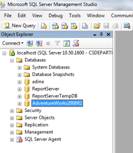
You will need a database and
some data some data to play with. For this lab we will use one of the SQL
Server sample databases. We will use the same database as in Lab 3 OLAP and
Lab5 Clustering. If you don't have it already on your computer, follow these steps:
1. Download the AdventureWorksDW_DATA.mdf
from the course website Lab 3 date and save it on your computer (desktop is
OK).
2. After you connect to (local)
using SQL Server Management Studio, right-click on "Databases"->
attach

3. Click on "Add" and browse to the desktop to find the file you downloaded.
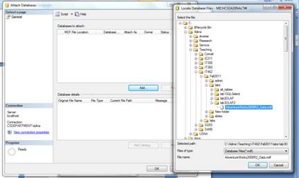
4. On the bottom side of the screen, select the "log" file and click on "Remove".

5. AFTER the log file is removed, click OK. The database should now show up in the list of databases on your server.
6. Create a file named yourlastname_Lab6.doc. You will be adding the answers to some
questions and a couple of screen shots to it.
Part 1 (Training a decision tree manually)
Create a small example data set that has two input attributes and one binary output attribute, e.g., with values Y and N. Choose the data records in the following way: When running the tree induction algorithm until each leaf is 100% pure (either all records in a leaf are of class N or all are of class Y), your tree should have at least two non-leaf nodes. You can achieve this with very few training records. Remember, you are training the tree by hand, so the fewer data records you use, the less time this will take.
Using your example data, train a decision tree by following the tree training algorithm we discussed in class, starting with the entire data set at the root node. Compute the information gain for each attribute and select the split with the greatest information gain for the root node. Repeat this process recursively in the next level. Remember, you just need one more split node (other than the root), so you want to keep your data set very small. Stop tree growing when each leaf node has a 100% pure data subset.
Show the final tree and all your work in constructing the tree.
Part 2 (Use
a Decison Tree in SQL Server Business Intelligence
Development Studio)
In Part 2
of the previous lab you learned how to create a data mining structure and a
data mining model with SQL Server Business Intelligence Development Studio. You
now have 2 options:
Option 1:
If you
still have the project you created for part 2 in previous lab, you can follow
the next steps to add a new mining model to the same project
To add a decision
tree model to an existing data mining structure:
- Open SQL Server Business Intelligence Development Studio.
- Click on File-> Open->Project/Solution. Browse to the mXXXXXX_Clustering project you created in previous lab and click on mXXXXXX_Clustering.sln file. Click on Open
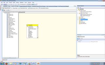
- Double-click on the mXXXXXX_Trageted Mailing Mining Structure that you created in the previous lab.
- Switch to the Mining Models tab in Data Mining Designer in Business Intelligence Development Studio.
Notice that the designer displays two columns, one for the mining structure and one for the TM_Clustering mining model, which you created in the previous lab.
- Right-click the Structure column and select New Mining Model.
- In the New Mining Model dialog box, in Model name, type TM_Decision_Tree.
- In Algorithm name, select Microsoft Decision Trees.
- Click OK.
Option 2:
If you do
not have the project you created for part 2 in previous lab, go to the previous
lab writeup and follow the steps in part 2 up to the
Processing Models part, but use the Microsoft Decision Tree algorithm rather
than Microsoft Clustering algorithm when creating the model. Name your model TM_Decision_Tree
You should now have a project with a Mining Structure containing the TM_Decision_Tree model in it.
Processing Models
in the Targeted Mailing Structure
Before you can browse or work with the mining model that you have created, you must deploy the Analysis Services project and process the mining structure and the mining model. Deploying sends the project to a server and creates any objects in that project on the server. Processing is the step, or series of steps, that populates Analysis Services objects with data from relational data sources. Models cannot be used until they have been deployed and processed.
![]() In
Data Mining Designer, you can process a mining structure, a specific mining
model that is associated with a mining structure, or the structure and all the
models that are associated with that structure. For this task, we will process
the structure and all the models at the same time.
In
Data Mining Designer, you can process a mining structure, a specific mining
model that is associated with a mining structure, or the structure and all the
models that are associated with that structure. For this task, we will process
the structure and all the models at the same time.
To deploy the project and process the mining model
1. In the Mining Model menu, select Process Mining Structure and All Models. (The "recycle" button)
If you made changes to the structure, you will be prompted to build and deploy the project before processing the models. Click Yes.
2. Click Run in the Processing Mining Structure - mXXXXXX_Targeted Mailing dialog box.
The Process Progress dialog box opens to display the details of model processing. Model processing might take some time, depending on your computer.
3. Click Close in the Process Progress dialog box after the models have completed processing. It is OK if the processing is complete with warnings, as long as you do not get errors.
4. Click Close in the Processing Mining Structure - <structure> dialog box.
Exploring the Decision
Tree Model
The Microsoft Decision Trees algorithm predicts which columns influence the decision to purchase a bike based upon the remaining columns in the training set.
The Microsoft Decision Tree Viewer provides the following tabs for use in exploring decision tree mining models: Decision Tree and Dependency Network.
![]() Decision
Tree Tab
Decision
Tree Tab
On the Decision Tree tab, you can examine all the tree models that make up a mining model.
Because the targeted mailing model in this project contains only a single predictable attribute, Bike Buyer, there is only one tree to view. If there were more trees, you could use the Tree box to choose another tree.
To explore the model in the Decision Tree tab
1. Select the Mining Model Viewer tab in Data Mining Designer.
By default, the designer opens to the first model that was added to the structure -- in this case, TM_Decision_Tree.
2. Use the magnifying glass buttons to adjust the size of the tree display.
By default, the Microsoft Tree Viewer shows only the first three levels of the tree. If the tree contains fewer than three levels, the viewer shows only the existing levels. You can view more levels by using the Show Level slider or the Default Expansion list.
3. Slide Show Level to the fourth bar.
4. Change the Background value to 1.
By changing the Background setting, you can quickly see the number of cases in each node that have the target value of 1 for [Bike Buyer]. Remember that in this particular scenario, each case represents a customer. The value 1 indicates that the customer previously purchased a bike; the value 0 indicates that the customer has not purchased a bike. The darker the shading of the node, the higher the percentage of cases in the node that have the target value.
5. Place your cursor over the node labeled All. An tooltip will display the following information:
o Total number of cases
o Number of non bike buyer cases
o Number of bike buyer cases
o Number of cases with missing values for [Bike Buyer]
Alternately, place your cursor over any node in the tree to see the condition that is required to reach that node from the node that comes before it. You can also view this same information in the Mining Legend.
6. Click on the one of the “Age” nodes. The histogram is displayed as a thin horizontal bar across the node and represents the distribution of customers in this age range who previously did (pink) and did not (blue) purchase a bike.
Based on the
tree, what attribute is the most important in predicting bike buying? Write your answer to yourlastname_Lab6.doc.
Based on the tree, what customers are likely
to purchase a bike? Write your answer to yourlastname_Lab6.doc.
Take a screen shot of the Decision
Tree viewer showing the tree and add it to yourlastname_Lab6.doc
Because you enabled drillthrough when you created the structure and model, you can retrieve detailed information from the model cases and mining structure, including those columns that were not included in the mining model (e.g., emailAddress, FirstName).
To drill through to case data
1. Right-click a node, and select Drill Through then Model Columns Only.
The details for each training case are displayed in spreadsheet format. These details come from the vTargetMail view that you selected as the case table when building the mining structure.
2. Right-click a node, and select Drill Through then Model and Structure Columns.
The same spreadsheet displays with the structure columns appended to the end.
Dependency Network Tab
The Dependency Network tab displays the relationships between the attributes that contribute to the predictive ability of the mining model.
To explore the model in the Dependency Network tab
1. Click the Bike Buyer node to identify its dependencies.
The center node for the dependency network, Bike Buyer, represents the predictable attribute in the mining model. The pink shading indicates that all of the attributes have an effect on bike buying.
2. Adjust the All Links slider to identify the most influential attribute.
As you lower the slider, only the attributes that have the greatest effect on the [Bike Buyer] column remain. By adjusting the slider, discover what two attributes are the greatest factors in predicting whether someone is a bike buyer.
What two attributes are the greatest factors
in predicting whether someone is a bike buyer? Write your answer to
yourlastname_Lab6.doc. Take a screen shot of the Dependency Network tab view
used to answer this question and add it to yourlastname_Lab6.doc
Testing Models
Now that you have processed the model by using the targeted mailing scenario training set, you will test your models against the testing set. Because the data in the testing set already contains known values for bike buying, it is easy to determine whether the model's predictions are correct. The model that performs the best will be used by the Adventure Works Cycles marketing department to identify the customers for their targeted mailing campaign.
You will test your model by making predictions against the testing set. Analysis Services provides a variety of methods to determine the accuracy of mining models. For now we will take a look at a lift chart.
On the Mining Accuracy Chart tab of Data Mining Designer, you can calculate how well each of your models makes predictions, and compare the results of each model directly against the results of the other models, if more than one model is present (for example, if you have both TM_Clustering and TM_Decision_Tree in this project). This method of comparison is referred to as a lift chart. Typically, the predictive accuracy of a mining model is measured by either lift or classification accuracy. We will use lift chart for now. For more information about lift charts and other accuracy charts, see Tools for Charting Model Accuracy (Analysis Services - Data Mining).
![]() Choosing
the Input Data
Choosing
the Input Data
The first step in testing the accuracy of your mining models is to select the data source that you will use for testing. You will test how well the models perform against your testing data and then you will use them with external data.
To select the data set
1. Switch to the Mining Accuracy Chart tab in Data Mining Designer in Business Intelligence Development Studio and select the Input Selection tab.
2. In the Select data set to be used for Accuracy Chart group box, select Use mining structure test cases to test your models by using the testing data that you set aside when you created the mining structure.
![]() Selecting
the Models, Predictable Columns, and Values
Selecting
the Models, Predictable Columns, and Values
The next step is to select the models that you want to include in the lift chart, the predictable column against which to compare the models, and the value to predict.
To show the lift of the model(s)
1. On the Input Selection tab of Data Mining Designer, under Select predictable mining model columns to show in the lift chart, select the checkbox for Synchronize Prediction Columns and Values.
2. In the Predictable Column Name column, verify that Bike Buyer is selected for each model.
3. In the Show column, select each of the models, if more than one are available.
4. In the Predict Value column, select 1. The same value is automatically filled in for each model that has the same predictable column.
5. Select the Lift Chart tab to display the lift chart.
When you click the tab, a prediction query runs against the server and database for the mining structure and the input table or test data. The results are plotted on the graph.
When you enter a Predict Value, the lift chart plots a Random Guess Model as well as an Ideal Model. The mining models you created will fall between these two extremes; between a random guess and a perfect prediction. Any improvement from the random guess is considered to be lift.
6. Use the legend to locate the colored lines representing the Ideal Model and the Random Guess Model.
Take a screen shot of the lift chart containg the TM_Decision_Tree
model and add it to yourlastname_Lab6.doc.
Creating and
Working with Predictions
You have trained, tested, and explored the data mining model you created. Now you are ready to use the model to identify recipients for Adventure Works Cycles targeted mailing campaign. You will now create a query to predict which customers are most likely to purchase a bike. You will also retrieve the probability that the prediction is correct, so that you can decide whether to present the recommendation to the marketing department or not.
Creating Predictions
After you have tested the accuracy of your mining models and decided that you are satisfied with them, you can then create Data Mining Extensions (DMX) prediction queries by using the Prediction Query Builder on the Mining Model Prediction tab in the Data Mining Designer.
The Prediction Query Builder has three views. With the Design and Query views, you can build and examine your query. You can then run the query and view the results in the Result view.
Before creating the query, lets add a column to the ProspectiveBuyer table:
1. In Solution Explorer, right-click the Targeted Mailing data source view and select View Designer.
2. Right-click the ProspectiveBuyer table title and select New Named Calculation.
3. In the Column name box, type calcAge.
4. In the Expression box, type DATEDIFF(YYYY,[BirthDate],getdate()), and then click OK.
The input table has no corresponding Age column. This expression will calculate customer age from the input table BirthDate column. Since Age was identified as one of the most influential column for predicting bike buying, it should exist in both the model and in the input table.
.
![]() Creating
the Query
Creating
the Query
The first step in creating a prediction query is to select a mining model and input table.
To select a
model and input table:
1. On the Mining Model Prediction tab of Data Mining Designer, in the Mining Model box, click Select Model.
2. In the Select Mining Model dialog box, navigate through the tree to the Targeted Mailing structure, expand the structure, select TM_Decision_Tree, and then click OK.
3. In the Select Input Table(s) box, click Select Case Table.
4. In the Select Table dialog box, in the Data Source list, select Adventure Works DW (or whatever name you gave to your data source for this project).
5. In Table/View Name, select the ProspectiveBuyer (dbo) table, and then click OK.
The ProspectiveBuyer table most closely resembles the vTargetMail case table.
![]() Mapping
the Columns
Mapping
the Columns
|
After you select
the input table, Prediction Query Builder creates a default mapping between
the mining model and the input table, based on the names of the columns. At
least one column from the structure must match a column in the external data. |
To map the
structure columns to the input table columns:
5. Right-click the lines connecting the Mining Model window to the Select Input Table window, and select Modify Connections.
Notice that not every column is mapped. We will add mappings for several Table Columns.
6. Under Table Column, click the Bike Buyer cell and select ProspectiveBuyer.Unknown from the dropdown.
This maps the predictable column, [Bike Buyer], to an input table column.
7. Under Table Column, click the Age cell and select ProspectiveBuyer.calcAge from the dropdown.
8. Click OK.
![]() Designing
the Prediction Query
Designing
the Prediction Query
To design the
prediction query:
1. The first button on the toolbar of the Mining Model Prediction tab is the Switch to design view / Switch to result view / Switch to query view button. Click the down arrow on this button, and select Design.
2. In the grid on the Mining Model Prediction tab, click the cell in the first empty row in the Source column, and then select Prediction Function.
This specifies the target column for the PredictProbability function. For more information about functions, see Data Mining Extensions (DMX) Function Reference.
3. In the Prediction Function row, in the Field column, select PredictProbability.
4. From the Mining Model window above, select and drag [Bike Buyer] into the Criteria/Argument cell.
When you let go, [TM_Decision_Tree].[Bike Buyer] appears in the Criteria/Argument cell.
5. Click the next empty row in the Source column, and then select TM_Decision_Tree.
6. In the TM_Decision_Tree row, in the Field column, select Bike Buyer.
7. In the TM_Decision_Tree row, in the Criteria/Argument column, type =1.
8. Click the next empty row in the Source column, and then select ProspectiveBuyer.
9. In the ProspectiveBuyer row, in the Field column, select ProspectiveBuyerKey.
This adds the unique identifier to the prediction query so that you can identify who is and who is not likely to buy a bicycle
10. Add five more rows to the grid. For each row, select ProspectiveBuyer as the Source and then add the following columns in the Field cells:
o calcAge
o LastName
o FirstName
o AddressLine1
o AddressLine2
Finally, run the query and browse the results.
To run the query and view results
1. In the Mining Model Prediction tab, select the Result button.
2. After the query runs and the results are displayed, you can review the results.
The Mining Model Prediction tab displays contact information for potential customers who are likely to be bike buyers. The Expression column indicates the probability of the prediction being correct. You can use these results to determine which potential customers to target for the mailing.
3. Click Save to save the results.
Copy the
contact information of the top 10 potential buyers or take a screen shot of the
Mining Model Prediction tab with this information and paste it into
yourlastname_lab6.doc.
Part 3:
a) In your Microsoft SQLServer database on cardhu.cs.usna.edu create a table to contain the sample data you created in Part 1. Make sure you add one extra column to be the primary key for the table (you can use IDENTITY(1,1) to have the content of that column generated by the DBMS).
b) Create a Business Intelligence Service project to connect to your cardhu database (use SQL Server Authentication with your username mXXXXXX and password) and create a decision tree mining model for the table you created. Check, and if needed modify, the parameters for the Microsoft Decision Tree algorithm (Right-click the TM_Decision_Tree model in Mining Models view and choose Set Algorithm Parameters option). Make sure your project is using the information gain as splitting criteria (Entropy).
Take a screen shot of
the screen showing the algorithm parameters changed to use Entropy and add it
to yourlastname_Lab6.doc.
Process and deploy your decision tree model and check whether the tree obtained by the Microsoft Decision Tree algorithm corresponds to the tree manually constructed by you in Part 1.
Did you obtain the
same tree as in Part 1? Why? Write your answers to yourlastname_Lab6.doc.
Take a screen shot of
the Decision Tree viewer for your data and add it to yourlastname_Lab6.doc.
Turn in:
Electronic:
- Upload
the file yourlastname_Lab6.doc with answers to Part 1 (if you have an
electronic version - paper version OK otherwise), Part 2, and Part3 to Blackboard.
- Upload
the zipped Business Intelligence Projects for Part 2 and Part 3.
Hard-copies:
- The completed assignment coversheet. Your comments will help us improve the course.
- Hard copy of yourlastname_Lab6.doc