IO and disk scheduling

3 kinds of I/O Devices - human interaction, machine interaction, and communication.
Differ in data rate, unit of transfer, representations, error types.
These differences make consistent models hard to achieve.
Disk Scheduling

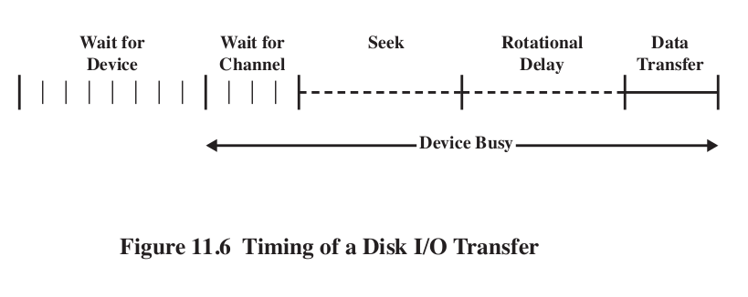
\[ T=\frac{b}{rN} \] Where T is transfer time, b is number of bytes, r rotation speed, N is number of bytes in track. \[ T_a = T_s + \frac{1}{2r}+\frac{b}{rN} \] This equation shows the penalty for accessing arbitrary locations on disk.
Try these on 55, 58,39,18,90,160,150,38,184.
LOOK is SCAN, bu we automatically wrap around when nothing else is in our way.
RAID. RAIDs are one of those counter-intuitive-but-brilliant ideas.
1. It stands for redundant array of inexpensive disks. The basic ideas is that with multiple disks, we can parallelize our reads.
2. But in this case locality is not our friend. If we spread our data across many disks, then at any one time we might be reading from just one of them anyway.
3. Instead, we make the disks redundant repeating on the multiple disks.
4. More disks means more disks likely to break. We must manage that.
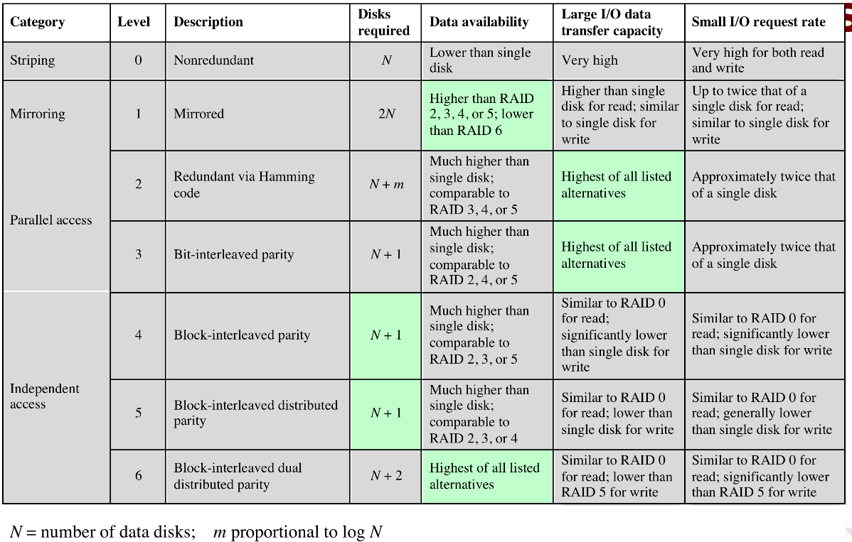
5. RAIDs can be executing in a number of ways, traditionally referred to as 'levels' 0-6.
6. RAID 0:
  1. Not really a RAID. Data is spread across all the disks, no redundancy.
  2. But data is not just spread around, it is striped. This helps with our locality. Making the strips small helps.
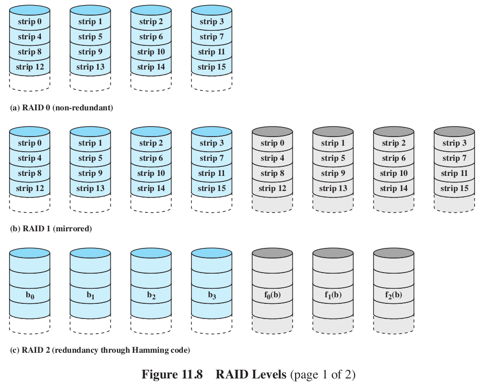
7. Level 1: Mirrored.
  1. This gives us some parallelism. Writes have to be done on both disks. Failure recovery is easy.
  2. Is however, expensive.
8. Level 2: Hamming code.
  1. All disks participate in every read. Stripes are super small (like a byte or 4).
  2. Use some of the disks to store the Hamming code for the stripe.
    1. Insert extra bits at positions that are powers of 2: 1,2,4,8,16,32. Values at those positions are computed as parities of the subset of bits:
    2. \(h_1(w)\) computes the parity of every other bit in the word: 1,3,5,7,9,...
    3. \(h_2(w)\) 2,3,6,7,10,11,...
    4. \(h_4(w)\) 4,5,6,7,12,13,14,15,...
    5. \(h_8(w)\) 8-15,24-31,...
    6. 011100101110 has a bit flipped. Where?
  3. still requires \(\log_2 w\) extra space.
9. Level 3:
  1. Similar to RAID 2, but with just 1 redundant disk.
  2. Parity bit set on the redundant disk based on xor of the bits on the other disks: \(X_r(i) = X_1(i) \oplus X_2(i) \oplus X_3(i) \oplus ... \)
  3. if disk 3 goes bad, when we replace it, we recompute its bits: \(X_3(i) = X_1(i) \oplus X_2(i) \oplus X_r(i) \oplus ... \)
  4. The machine can even keep running with disk failure, because we could do the parity computation on the fly.
  5. Very high transfer rates for big moves.
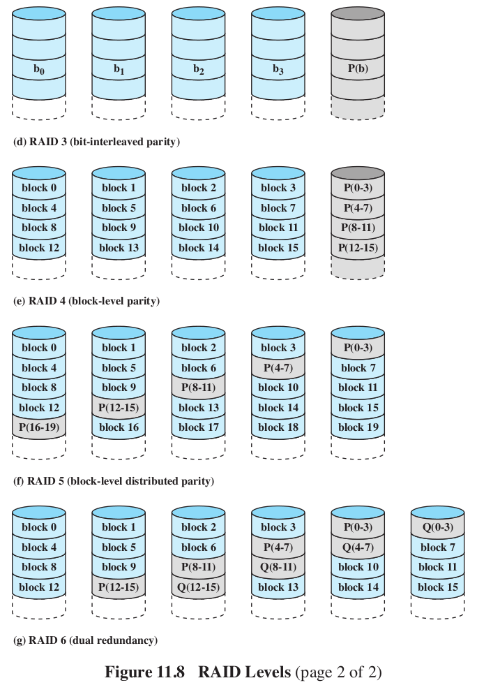
10. Level 4:
  1. Make the strips bigger. That's it.
11. Level 5:
  1. Distribute the parity, so we don't have to write to the same parity disk every time we write.
12. Level 6:
  1. Like 5, but now with two parity checks per bit.
  2. one is xor
  3. The other is more complex, essentially encryption.
  4. Can reconstruct the data even with the loss of 3 disks.
Disk Cache
1. Just like a RAM cache, but for disks.
2. Locality!
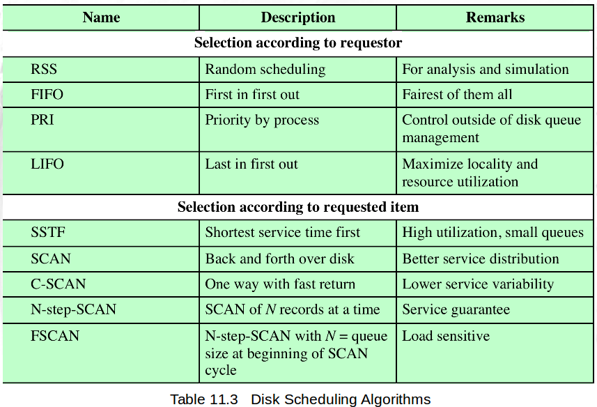
3. The question we always ask is, what disk sector gets swapped out?
4. Least Recently Used. Sound familiar?
5. Least Frequently Used. Keep a count of the references. Move out the one with the smallest number.
6. LFU has a problem- if a block is used in burst (many accesses in a row, followed by long periods of inactivity) then the counts will still be high enough to keep it from being swapped out, even though it is not going to be used in a while.
7. Solution: only increment counters if it has not recently been incremented.
Linux
1. Special files are associated with each device. You can read and write from them like a file.
2. Two kinds of devices- Character and block. character devices have no caching, block devices do. Many can be opened in either mode.
3. There are 3 disk schedulers: the Elevator Scheduler (a variation of LOOK), Deadline Scheduler, and Aniticipatory I/O.
4. Elevator:
  1. if new request is same or adjacent to something on the queue, merge the two
  2. If any request on the queue is older than a threshhold, new requests are added to tail.
  3. Else, place in sorted order,
5. Deadline:
  1. 2 above addresses starvation, but not super effective (wrong pokemon type? No, write requests (which no one blocks on, could crowd out read requests)
  2. New requests are put in either a FIFO read queue or FIFO write queue, plus the elevator queue.
  3. Each request has a deadline- 5 second fro write, 0.5 for read.
  4. Normally select job from Elevator, but if head of either FIFO queue has expired, then select from it.
6. Anticipatory
  1. If process is reading with short delays, we might jump to servicing another request, and then come back to to this read, which was close to where we were before.
  2. When a read request is dispatched from the FIFO read queue, the scheduling system pauses for 6ms afterthe read to see if anything else is coming from that process.
  3. A little surprising that it is super effective.