Every election cycle features polling data from key Senate races. A cottage industry exists to interpret the polls and forecast the upcoming results. The 2022 midterm elections will determine which party controls the Senate, so this project challenges you to make your own forecast based on the polling data.
This is a project, not a lab, so the strict no-collaboration-policy is in place for this assignment. See the course policy. You must implement this project on your own without assistance from anyone else except your instructor and MGSP (and MGSP will operate under some new restrictions as well).
Milestone 1: Nov 15 (Steps 1+2)
Milestone 2: Dec 1 (Step 3)
Full Project: Dec 9
Each milestone is worth 5% of the project grade. Grace days may be used on milestones and/or full project.
Download the CSV files senate_polls.csv and states.csv.
(this data was pulled from fivethirtyeight.com)
1. Write a function create_state_dict(filename) that creates a dictionary from name to abbreviation by reading the states.csv file. We will draw a country map like the COVID lab, so we need state abbreviations ("MD") for the mapping library to understand. Our polling data uses full state names ("Maryland"), hence the need for this function.
2. Write a function get_polls(rows,state,party) that gets all polls for a party ("DEM") in one state ("Florida"). This function returns a dictionary. Each poll has a date on which it was completed. Use the 'end_date' column. Your function must loop over the rows from a DictReader that reads the polling file, and make a dictionary that maps datetime objects (datetime 10/30/22) to polling percentages (43.5).
Datetime usage reminder: today = datetime.strptime("11/01/22", '%m/%d/%y')
Create a file polling.py and copy in this starter code to test for correctness:
from datetime import datetime,timedelta
from csv import DictReader

# Define create_state_dict


# Define get_polls


# Don't change anything below here.
if __name__ == '__main__':
    state_to_abbrev = create_state_dict('states.csv')

    passed = 0
    for k,v in [('Ohio','OH'),('Florida','FL'),('Utah','UT'),('California','CA')]:
        if state_to_abbrev[k] == v:
            passed += 1
    if passed == 4:
        print('PASS state abbreviations')
    else:
        print('FAIL state abbreviations')

    # Test polls
    fh = open('senate_polls.csv')
    csv_reader = DictReader(fh)
    rows = list(csv_reader) # this reads all rows into one List!
    polls = get_polls(rows,'Ohio','DEM')

    ans = {datetime(2022, 11, 1, 0, 0): 44.1, datetime(2022, 10, 30, 0, 0): 43.7, datetime(2022, 10, 28, 0, 0): 43.1, datetime(2022, 10, 26, 0, 0): 42.0, datetime(2022, 10, 24, 0, 0): 44.2, datetime(2022, 10, 23, 0, 0): 50.2, datetime(2022, 10, 22, 0, 0): 43.3, datetime(2022, 10, 20, 0, 0): 45.0, datetime(2022, 10, 19, 0, 0): 46.0, datetime(2022, 10, 18, 0, 0): 43.2, datetime(2022, 10, 16, 0, 0): 43.0, datetime(2022, 10, 15, 0, 0): 45.0, datetime(2022, 10, 14, 0, 0): 42.8, datetime(2022, 10, 12, 0, 0): 43.8, datetime(2022, 10, 8, 0, 0): 44.4, datetime(2022, 10, 7, 0, 0): 44.7, datetime(2022, 10, 3, 0, 0): 49.0, datetime(2022, 9, 22, 0, 0): 46.0, datetime(2022, 9, 15, 0, 0): 45.0, datetime(2022, 9, 13, 0, 0): 40.1, datetime(2022, 9, 11, 0, 0): 46.1, datetime(2022, 9, 7, 0, 0): 46.6, datetime(2022, 9, 2, 0, 0): 44.0, datetime(2022, 8, 23, 0, 0): 50.0, datetime(2022, 8, 18, 0, 0): 44.9, datetime(2022, 8, 16, 0, 0): 41.6, datetime(2022, 8, 3, 0, 0): 49.0, datetime(2022, 7, 28, 0, 0): 48.0, datetime(2022, 7, 24, 0, 0): 44.0, datetime(2022, 7, 3, 0, 0): 41.0, datetime(2022, 6, 30, 0, 0): 48.0, datetime(2022, 5, 24, 0, 0): 39.4, datetime(2022, 5, 13, 0, 0): 37.0, datetime(2021, 8, 24, 0, 0): 36.0, datetime(2021, 3, 19, 0, 0): 42.0}
    if polls == ans:
        print('PASS get polls')
    else:
print('FAIL get polls') Create a file query.py for a simple user interface. Your program will run like so:
State? Utah
Party (DEM/REP)? DEM
2022-02-14 00:00:00	25.0
2022-03-21 00:00:00	11.0
2022-03-24 00:00:00	13.0
AVG: 16.33
DECAY AVG: 12.54
You will import your polling.py functions, call get_polls() based on the user's query, and retrieve the dictionary that maps dates to poll results. You must print them in sorted order (see above!).
Observe the AVG and DECAY AVG numbers after the sorted print. You must write two functions that compute these values.
\(avg = \frac{1}{N} \sum_i p_i \)
Example decay (today = Nov 1 2022)
poll 1: Sep 15 2022 with 40%
poll 2: Oct 1 2022 with 44%
poll 3: Oct 20 2022 with 48%
basic = 44.0% (basic avg)
timedecay = \( \frac{.6^{6.7}*40 + .6^{4.4}*44 + .6^{1.7}*48}{.6^{6.7} + .6^{4.4} + .6^{1.7}} \) = 46.77%
\(avg = \frac{1}{\sum_i \alpha_i} \sum_{i} (\alpha_i*p_i) \)
The \(\alpha\) variables are the decay factors, each computed based on how many weeks have passed since the poll occurred:
\( d = 0.6 \) # hard-code this weekly decay factor
\( \alpha_i = d^{weeksSincePoll} \)
In other words, if a poll was 44% and occurred today, then \(\alpha_i = 1\) and it's still 44. However, if it occurred two weeks ago, then \(\alpha_i = 0.6^2 = 0.36\) which you then multiply by 44% to get the weighted result (\(0.36*44=15.84\)). Note that the number of weeks will be a float. Calculate how many days ago the poll was, then divide by 7.
Calculating time distances with datetime objects:
# If we have two dates
today = datetime.strptime("11/01/22", '%m/%d/%y')
pastday = datetime.strptime("10/01/22", '%m/%d/%y')

# We can just subtract
elapsed_time = today - pastday

# Use the days variable in the elapsed datetime object
elapsed_days = elapsed_time.days
print('This many days have passed', elapsed_days)
As you write your solution, follow these guidelines:
Start from this starter code:
# Your function definitions here.


if __name__ == '__main__':
    # Today is Nov 1, 2022
    today = datetime.strptime("11/01/22", '%m/%d/%y')

    # Your program's main logic here.
Define and use the function forecast_basic(polls)
Define and use the function forecast_decay(polls)
Use round(margin,2) before printing to only show decimals.
A longer expected output is shown here:
State? Florida
Party (DEM/REP)? DEM
2021-06-27 00:00:00	39.6       <--- one tab character '\t' between the date and number
2021-08-10 00:00:00	39.0
2021-08-17 00:00:00	46.1
2021-08-18 00:00:00	45.1
2021-08-24 00:00:00	33.0
2021-09-27 00:00:00	38.0
2021-10-23 00:00:00	28.6
2021-11-09 00:00:00	34.0
2021-11-19 00:00:00	44.3
2022-01-29 00:00:00	41.4
	...
	...
2022-09-20 00:00:00	47.0
2022-09-25 00:00:00	41.0
2022-09-27 00:00:00	46.0
2022-09-28 00:00:00	41.0
2022-10-13 00:00:00	45.0
2022-10-16 00:00:00	42.0
2022-10-20 00:00:00	45.0
2022-10-23 00:00:00	44.0
2022-10-24 00:00:00	43.0
AVG: 40.87
DECAY AVG: 43.7
Create a file predict.py. Starter code is below.
Take note of the functions you have working from previous steps. These are your tools:
You are ready to make polling predictions for states. We provide you a list of battleground states:
STATES = ['Arizona','Colorado','Connecticut','Florida','Georgia','Illinois','Indiana','Iowa','Kansas','Missouri','Nevada','New Hampshire','New York','North Carolina','Ohio','Oregon','Pennsylvania','Utah','Washington','Wisconsin']
Your task is to loop over these states, get the DEM/REP decayed polling averages for each state (use Nov 1,2022 as today for the decay), and print out your predicted margins (margin = REP - DEM). Use round(margin,2) before printing to only show two past the decimal:
AZ -4.08
CO -11.54
CT -12.2
FL 6.98
GA 0.27
IN 2.08
IL -13.46
IA 8.37
KS 21.1
MO 11.47
NV 0.94
NH -1.56
NY -15.26
NC 2.16
OH 1.88
OR -12.91
PA -1.12
UT 35.66
WA -5.63
WI 2.69
In order to do this, define a function compute_state_margins(rows) that takes your DictReader's rows, and returns a dictionary from state abbreviation ('PA') to REP-DEM margin of victory (-4.25). Call your other functions from this to accomplish your task. Loop over all states and put their margins in the dictionary, then return the dictionary.
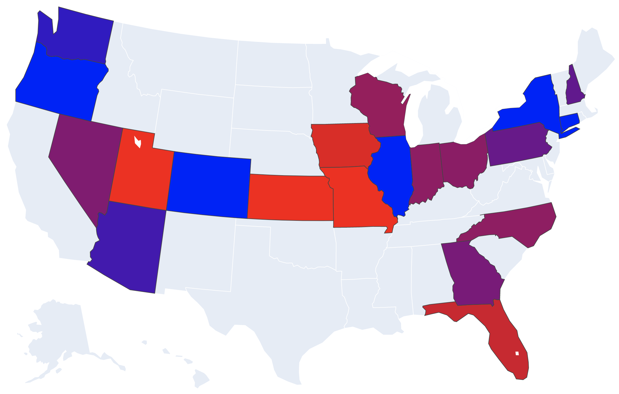
When you have the above working, visualize it! Create a states list and a values list from your margins dictionary, and send it to the map just like we did in the COVID lab. This time I've chosen blue/red colors for the political parties, with purple at a margin of 0.0:
STATES = ['Arizona','Colorado','Connecticut','Florida','Georgia','Indiana','Illinois','Iowa','Kansas','Missouri','Nevada','New Hampshire','New York','North Carolina','Ohio','Oregon','Pennsylvania','Utah','Washington','Wisconsin']

# FILL IN THIS FUNCTION
def compute_state_margins(rows):


if __name__ == '__main__':
    import plotly.express as px

    # YOUR CODE HERE (call compute_state_margins, and use its returned dictionary)


    # Create the map object -- fill the STATE_ABBREVS and VALUES variables here.
    fig = px.choropleth(locationmode="USA-states", scope="usa", color_continuous_scale=[(0,'blue'),(1,'red')],
                        range_color=(-10,10),
                        locations=STATE_ABBREVS, color=VALUES)
    # Show the map in a web browser.
    fig.show()
Your map should look like the picture at the top of this step!
Make one small addition to the end of your program. Count the number of REP and DEM victories in these 20 battleground states (using the margins). Add them to the other 80 states which we aren't showing -- they have 40 Rs and 40 Ds (we're counting Independents as Democrats because they currently caucus with the Democrats). Print out the result after your current output:
PREDICTION: 51 Rs 49 Ds
Make a small change to your compute_state_margins(rows) function.
Change the definition to accept a polling bias float: compute_state_margins(rows,dembias)
This will be a number, like 1.1, which indicates how biased toward (or away from) the democrats the polls are. If a poll reports 44% D and 42% R at a +2% D margin -- but there is a +1.1% democrat bias -- then the true D margin is +0.9% (43.45% D and 42.55% R). Your task is to change your function so that it takes the bias into account. You likely will change just one line of code where you compute the (REP-DEM) margin. Yes, the bias might be negative, which means it is biased toward the republicans.
Try sending in different biases and see how your predictions change! Set it to 1.1 to turn it in. You should see all your scores change by 1.1. Does the final prediction change?
AZ -2.98
CO -10.44
CT -11.1
FL 8.08
GA 1.37
IN 3.18
IL -12.36
IA 9.47
KS 22.2
MO 12.57
NV 2.04
NH -0.46
NY -14.16
NC 3.26
OH 2.98
OR -11.81
PA -0.02
UT 36.76
WA -4.53
WI 3.79
PREDICTION: 51 Rs 49 Ds
Copy predict.py to predictsim.py.
This last step explores polling bias and expected election results. The accuracy of polls is a hot topic amongst election nerds. Which polling agencies are most accurate? Is this election cycle different than past ones? What if all the polls have an incorrect bias toward one party?
We can look at past polling performance, and see what the bias is for each polling firm. Organizations like FiveThirtyEight have actually done this for most pollsters, exploring how they performed in past elections. They've calculated the average bias of each pollster. Professor Chambers took this data (450 pollsters!) and computed the mean bias across all of them (+1.1 toward democrats -- i.e., if Dems polled at 44 then the true number was 42.9) with the standard deviation (6.2). This means that historically for any given pollster, you might presume they are 1.1 incorrectly biased to favor Democrats (but with a big standard deviation).
In this section, you will simulate your Step 3 prediction with different biases, checking to see when your predictions change if the bias shifts.
WHAT TO DO:
Where do you get 200 polling biases? You will sample the actual pollster distribution from historic performance! We found that the mean bias is 1.1 with one standard deviation at 6.2. Python can sample from a normal distributions like this:
import numpy
numpy.random.seed(SEED_VALUE) # set this from the user ONCE at the start of your program
dembias = numpy.random.normal(1.1,6.2)
Loop 200 times, sample a new Democrat bias (it might be negative, which is a republican bias), and keep track of your predictions. Print the average of all runs.
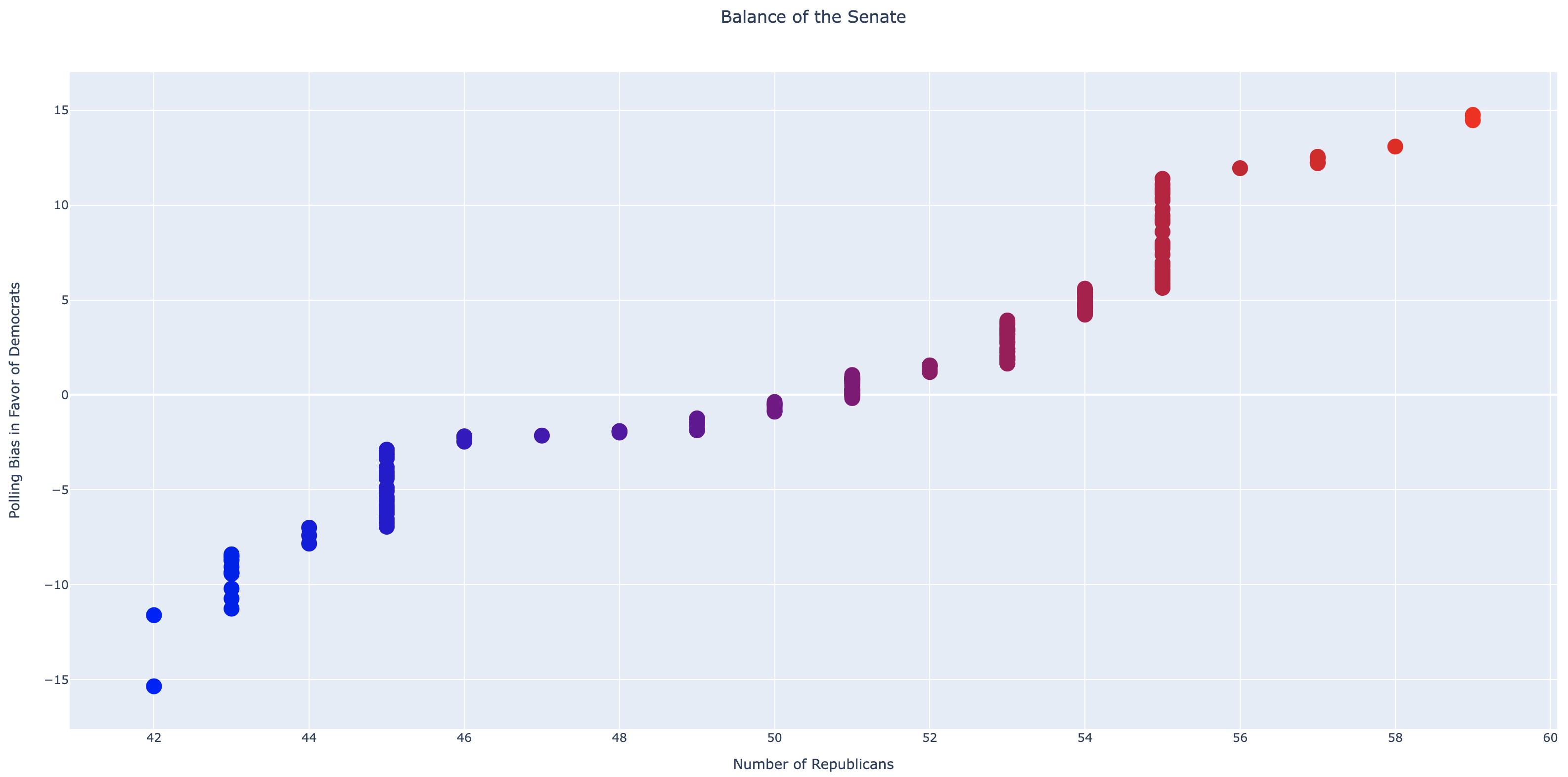
Finally, visualize all of these predictions (see the picture in this section). You should have two lists of numbers now: (1) LIST_OF_REPS (how many predicted republicans each time), and (2) BIASES (the bias used each time). We will use the Plotly library again for visualizing, and you can see how to do that here:
import plotly.graph_objects as go
fig = go.Figure(data=go.Scatter(x = LIST_OF_REPS, y = BIASES, mode='markers',
                marker=dict(size=16, color=LIST_OF_REPS, colorscale=[(0,'blue'),(1,'red')])))
fig.update_layout(title='Balance of the Senate',title_x=0.5,
                  xaxis_title='Number of Republicans',yaxis_title='Polling Bias in Favor of Democrats')
fig.show()
Don't change the above sample code! Your job is to just fill the LIST_OF_REPS and BIASES lists beforehand.
Your program should follow this exact input and output (and also pop up the graphic!):
Polling data? senate_polls.csv
Seed? 11
Simulations? 200
PREDICTION (bias 11.95)	 56 Rs 44 Ds
PREDICTION (bias -0.67)	 50 Rs 50 Ds
PREDICTION (bias -1.9)	 48 Rs 52 Ds
PREDICTION (bias -15.35)	 42 Rs 58 Ds
PREDICTION (bias 1.05)	 51 Rs 49 Ds
PREDICTION (bias -0.88)	 50 Rs 50 Ds
PREDICTION (bias -2.23)	 46 Rs 54 Ds
PREDICTION (bias 3.06)	 53 Rs 47 Ds
	  ...
	  ...
PREDICTION (bias -9.36)	 43 Rs 57 Ds
PREDICTION (bias -9.42)	 43 Rs 57 Ds
PREDICTION (bias -1.45)	 49 Rs 51 Ds
PREDICTION (bias 0.82)	 51 Rs 49 Ds
PREDICTION (bias -1.33)	 49 Rs 51 Ds
PREDICTION (bias 10.61)	 55 Rs 45 Ds
PREDICTION (bias 0.08)	 51 Rs 49 Ds
PREDICTION (bias 3.33)	 53 Rs 47 Ds
AVERAGE: 50.56 Rs 49.44 Ds
Download the full pollster statistics CSV file.
Create a new program extra.py that is a copy of your last part. One big generalizing assumption we make is that the polling bias +1.1 is applied to all polls, even though we know the actual bias of individual pollsters. The 1.1 was an average of all.
Change your program so that instead of sampling from the normal distribution (1.1,6.2), you sample from each pollster's own mean. Replace 1.1 with the pollster's mean. Use the linked pollster CSV to get all pollsters and their bias (the 'Bias' column). You'll have to update how your program calls for the polls to send the correct bias to your function.
Have your program generate a new final Step chart.
Your three programs (polling.py, query.py, predict.py, and predictsim.py).
submit -c=sd211 -p=project polling.py query.py predict.py predictsim.py