State Space Search
Introduction to Intelligence and Search
Intelligence is fundamentally about making effective choices. To make a good choice, an agent must consider various alternatives and their potential effects. The systematic process of considering these alternatives is known as search.
A core hypothesis in AI is that all problems requiring intelligence can be formulated as a state space, where intelligence is demonstrated by searching within that space.
State Space Search
A problem is defined by its state space, which consists of the following four elements:
State: A specific condition or mode of the problem.
Initial State: The start state from which the program attempts to solve the problem.
Set of Operators: Actions available within the problem framework. An operator transitions the system from the current state to another valid state.
Goal State: The desired state the problem should end in.
Note: While usually interested in the specific sequence of operators (the path) required to reach the goal state, this is not always the case.
Examples of State Space Problems
Route Finding: Finding a path between two locations (e.g., from Michelson to Ram’s Head Tavern).
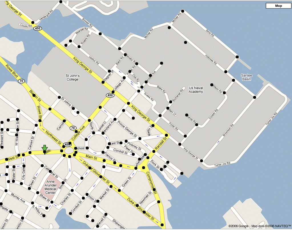
Annapolis waypoints. Find the shortest path using waypoints.
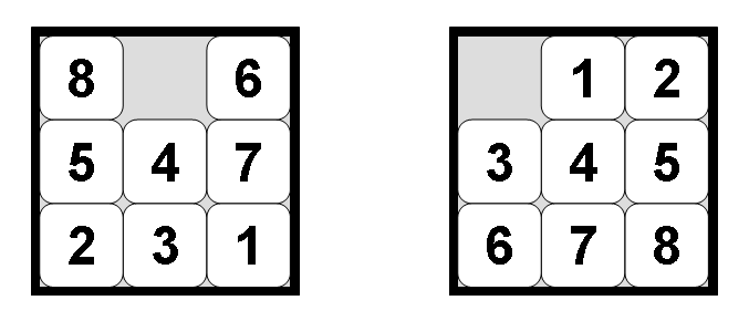
The 8-Puzzle (or 15-Puzzle): Moving tiles to achieve a target configuration.
Other Examples: Missionaries and Cannibals, Rubik’s Cube, Traveling Salesman (wiring), and Robot Path Planning.
These problems can all be mathematically modeled as a graph.
The Generate and Test Algorithm
The basic process of search involves “expanding” a state by generating its successors. Most search algorithms follow the generate-and-test model which is really just a general paradigm for searching a state space. You can think of it like this:
GenerateTest(StartState s)
  while (isNotGoal(s))
    generate successors to s
    point successors back to s
    add successors to the open set
    add s to the closed set
    s <- SOME state from open
State Space vs. Search Tree: It is important to distinguish between the state space and the search tree. Because algorithms may loop or undo previous operators, the resulting search tree is often significantly larger than the underlying state space. These graphs are implicit; rather than storing the entire graph in memory, the algorithm keeps only a portion in memory, implying the rest via the start state and our operators.
Search Algorithm Evaluation Criteria
When evaluating search algorithms, we consider four key metrics:
Completeness: Is the algorithm guaranteed to find a solution if one exists?
Optimality: Does the algorithm guarantee finding the optimal (best) solution?
Time Complexity: How long does it take to find a solution? This is typically measured in the worst-case scenario, though average-case is sometimes used.
Branching Factor: The average number of children per node.
Depth: The number of levels the algorithm searches through.
Space Complexity: How much memory does the algorithm require? In AI, memory constraints are often more critical than time constraints.
Brute-Force Search Strategies
Brute-force (or uninformed) search strategies do not use domain-specific knowledge to guide the search. The four we cover in this class are:
Breadth-first search
Uniform-cost search
Depth-first search
Bi-directional search
1. Breadth-First Search (BFS)
BFS expands the current node and then all of its children before moving deeper. It covers all nodes at depth 1, then depth 2, and so on. Pseudocode:
BreadthFirstSearch(StartState s)
  add s to closed
  while ( s != null and isNotGoal(s) )
    generate successors to s
    for each successor not in closed
      point successor back to s
      add successor to closed
      add successor to open queue
    s <- next state from open queue

  return s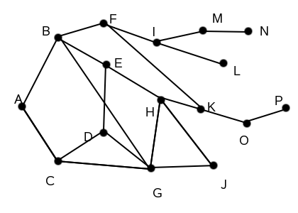
Basic graph. Example of a graph with nodes that you might search.
Example trace of the search:
| Open Queue | Closed List | Comment |
|---|---|---|
| (A) | Start at A | |
| (B A) (C A) | (A) | Add neighbors of A |
| (C A) (E B A) (F B A) (G B A) | (A B) | New states go to the back |
| (E B A) (F B A) (G B A) (D C A) | (A B C) | G already in open set |
| (F B A) (G B A) (D C A) (H E B A) | (A B C E) | Search continues... |
Analysis:
Complete: Yes.
Optimal: Yes (provided path costs are uniform).
Complexity: Assume branching factor b and solution at depth d:
Then the time it takes to find a solution at depth d is a factor of the number of nodes the algorithm generates to find that solution. If d=0, then the number of nodes is 1. If d=1, then the number of nodes is 1+b, and if d=2 then the number of nodes is 1+b+b^2. In general this becomes, for depth d: 1+b+b^2+b^3+...+b^d.
Time Complexity: Since the last term of the polynomial dominates, the time is O(b^d)
Space Complexity: How many nodes must be kept in memory at one time? The entire frontier (at least) must be kept in memory so the next level of the tree can be generated: O(b^d)
Both time and space complexity are exponential in the depth of the solution. This is very, very, nasty.
Scale of the Problem:
| Depth | Nodes | Time | Memory |
|---|---|---|---|
| 0 | 1 | .00001 sec | 100 bytes |
| 2 | 111 | .001 sec | 10 KB |
| 4 | 11,111 | .11 sec | 1 MB |
| 6 | 10 sec | 111 MB | |
| 8 | 17 min | 11 GB | |
| 10 | 28 hours | 1 TB | |
| 12 | 116 days | 111 TB | |
| 14 | 32 years | 11 PB |
What does this tell us? If the problem is big enough, then time can be a serious contstraint, BUT using BFS, the real problem is memory. I commonly have problems that take an hour or 2 to run, but 11G of RAM is not easy to come by even on today’s bigger machines. Serious problems are often worth waiting a week or 2 to run, but where are you going to get a terabyte? And that is only at depth 10.
2. Uniform-Cost Search
Uniform Cost is just like breadth-first search, except instead of expanding a node from the shallowest depth, you expand a node with the minimal cost accrued so far g(n).
Pseudocode:
UniformCost(StartState s)
  while ( s != null and isNotGoal(s) )
    add s to closed
    generate successors to s
    for each successor c not in closed
        calculate g(c)
        point c back to s
        add c to open priority queue
    s <- next state from open

  return s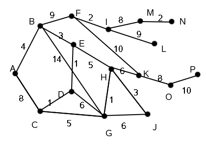
Graph with edge costs. Example of a graph with edges that have costs.
Key Notes on the Closed List:
Nodes must only be added to the closed list when they are expanded, not when generated.
If a node were added upon generation, the algorithm might discard a subsequent shorter path to that same node found later.
While the closed list could be omitted, doing so risks filling the priority queue with multiple copies of states, wasting space and computation.
Observations: This uniform cost search has similar characteristics of breadth-first search, except it works better for searches with costs. This is the famous Dijkstra’s algorithm.
Analysis:
Complete: Yes.
Optimal: Yes.
Time Complexity: O(b^(c*/e+1))
Space Complexity: O(b^(c*/e+1))
3. Depth-First Search (DFS)
DFS always expands the node deepest in the search tree. It utilizes a stack, and importantly for us, we do not use a CLOSED LIST! You may see DFS implementations elsewhere that use a closed list, but we will focus on a memory-efficient version that does not need it.
Pseudocode:
DepthFirstSearch(StartState s)
  while (s != null and isNotGoal(s))
    generate successors to s (not on this path)
    point successors back to s
    push each successor on open stack
    s <- pop next state from open
  return s
Basic graph. Example of a graph with nodes that you might search.
Example trace of depth-first search:
| Open Queue | Comment |
|---|---|
| (A) | |
| (B A) (C A) | not exciting yet |
| (E B A) (F B A) (G B A) (C A) | C is getting buried on the stack |
| (H E B A) (D E B A) (F B A) (G B A) (C A) | Can’t count on particular expansion order |
| (K H E B A) (J H E B A) (G H E B A) (D E B A) (F B A) (G B A) (C A) | hey, this isn’t the shortest path... |
| ... | ... |
Analysis:
Optimal: No.
Complete: Maybe (only if the search depth is limited or the space is finite).
Time Complexity: O(b^d)
Space Complexity: O(d) - this is a significant advantage over BFS.
4. Depth-First Iterative Deepening (DFID)
Depth-First Iterative Deepening (DFID) is an algorithm designed to combine the best properties of Depth-First Search and Breadth-First Search. It attempts to add optimality and completeness to DFS while maintaining its efficient space complexity.
The Strategy: Depth-Limited Search
To understand DFID, imagine a Depth-Limited DFS. This is a standard DFS that treats any node at a specific depth d as a dead end (a “cutoff”).
If the true minimal solution lies at depth s, running a DFS with a limit of d yields three possible outcomes:
s > d : The DFS will not find a solution (the cutoff is too shallow).
s < d : The DFS will find a solution, but it is not guaranteed to be optimal (it may find a deeper, non-optimal solution down a different branch first).
s = d : The DFS will find a solution, and it is guaranteed to be optimal.
Ideally, we would run a depth-limited DFS where the limit equals the exact depth of the solution (s=d). However, since we do not know the depth of the solution beforehand, we must find it iteratively.
The Algorithm
DFID proposes a simple iterative process:
Perform a depth-limited DFS with a limit of 0.
If a solution is found, terminate.
If not, increment the depth limit by 1 and start over.
Repeat this process until a solution is found.
Why this works:
Optimality: If we find a solution at depth n, we are certain it is the optimal solution. If a shallower solution existed, we would have found it during the previous iteration at limit n-1
Completeness: Given enough time, the depth limit will eventually reach the solution depth s, guaranteeing that the solution is found.
Space Complexity: At any given moment, we are strictly performing a DFS. Therefore, the space complexity remains O(d).
Time Complexity Analysis
But wait! Since we restart the search from scratch for every new depth limit, aren’t we doing a significant amount of redundant work?
Let’s analyze the number of nodes generated. Assume a branching factor b and a solution depth s.
In the final iteration (depth d), the nodes at the bottom level are generated once: b^d
The nodes at depth d-1 were generated in the current iteration and the previous iteration (total 2 times): 2b^(d-1).
The nodes at depth d-2 were generated in the current iteration, and the two previous iterations (total 3 times): 3b^(d-2)
Summing this up for the total search gives us: b^d + 2b^(d-1) + 3b^(d-2) + ... + db^0
While this looks like a lot of extra work, the total work is dominated by the largest term. This series is bounded by a polynomial where the dominant term is b^d
Conclusion: Despite the re-generation of upper levels, the asymptotic time complexity remains O(b^d).
DFID is often a “big win” for large search spaces requiring brute-force algorithms, as it achieves the low memory footprint of DFS with the optimality of BFS.
5. Bi-directional Search
The idea of bi-directional search is to reduce time while caring less about space. This strategy runs two simultaneous searches: one forward from the start state and one backward from the goal state. A solution is found when the two meet in the middle.
Completeness: yes, if even one of the searches is complete
Optimality: yes, if the two searches are individually optimal
Time Complexity: If the searches meet in the middle, the complexity is 2*b^(d/2) = O(b^(d/2))
Space Complexity: Depends on the searches. Could be O(d) for two DFS
Issues:
Can we go backwards? Not all problems can we figure out the previous state from the current one.
What if there are multiple goal states? What if the goal states are implicit?
Can we efficiently check if a given node is part of the frontier of the of other search? Yes, using a hash table. But then the frontier must be stored in that hash table. In order to guarantee that the 2 searches will meet at all, at least 1 must be BFS, thus the table size is bd/2 . Therefore, for any serious implementation of bi-directional, the space complexity is O(bd/2).
Partial Information Scenarios
In some cases, the agent lacks full knowledge of the state space:
Sensorless: The agent does not know its current state and must reason using sets of potential states, known as belief states.
Contingency: The results of actions are uncertain; if an action fails, the plan must adapt.
Exploration: The environment is unknown, requiring the agent to explore to learn the state space.