Optimization

Nearly everything we do in this class is some form of an optimization problem. These optimization problems primarily consist of a loss function or objective function ℒ(𝒟, w). This loss function is a mathematical combination of our data 𝒟 and our parameters w. For a given application, we design a loss function which communicates how well our solution is doing. For example, in K-Means clustering, our loss function was the total within-cluster variance, the data was the data points, and the w was our assignments of points to clusters.

In ML, we design these loss functions, and then count on mathematical and computational tools to find the w which result in the best possible version we can put together for our problem. Again revisiting K-Means, the K-Means algorithm resulted in the better and better cluster assignments until the loss function couldn’t seem to decrease any more; these assignments were our solution.

When we write optimization problems, we have to state a couple things aside from the loss function. First, we state whether we want our loss function to be big or small, by stating whether the goal is to minimize or maximize it. Second, we state the loss function. Third, we explicitly state which variables in the loss function we can control to perform this optimization. Finally, there may be some additional constraints on the solution.

It can be useful to visualize a loss function as a surface in space. For example, perhaps your loss function has two parameters. As you change those parameters, the loss function increases, or decreases, meaning the surface rises or falls. If minimizing the loss function, the goal is to find the spot on the surface with the smallest value. The properties of the optimization problem determine if this minimum point is easy or hard to find.

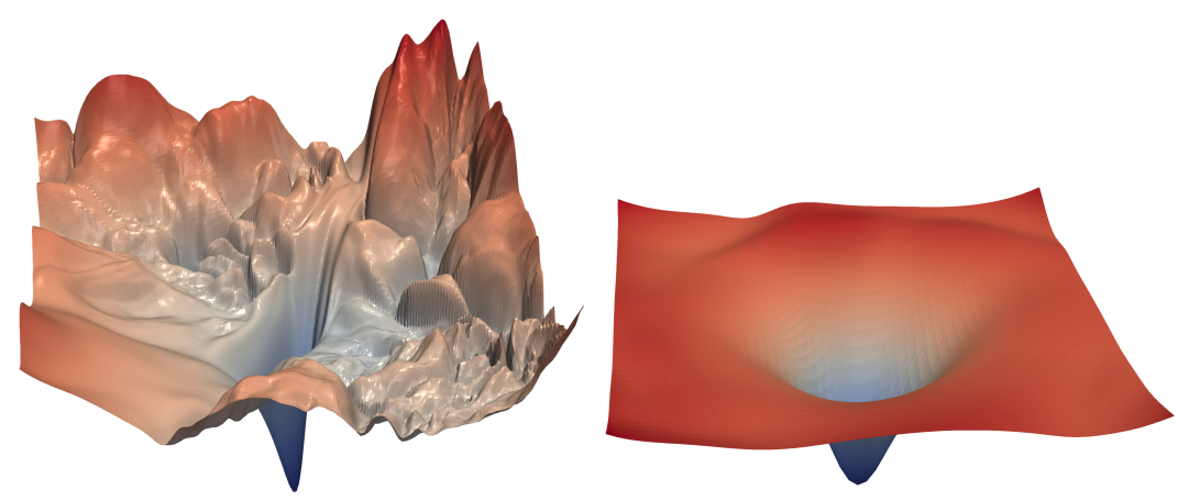Which would you rather optimize?

Fully understanding how we can solve these optimization problems is deeper than we can reasonably go in an undergraduate ML class. But, some context is important in understanding what your solutions might look like, and how long we can expect solutions to take.

From easiest to hardest, we can break these down into:

• Problems we can solve in closed form.
• Problems which are convex.
• Problems which are nonconvex.
• Problems which are discrete.

Closed Form

You have actually seen this before, repeatedly, in Calculus class, where you were asked to minimize or maximize a function. What did you do? You symbolically calculated the gradient of the function, set it equal to zero, then algebraically solved for your variables. This gave you a closed-form solution of the form w = something, where you could calculate the minimum exactly, without having to do any iterative algorithm. This is generally very fast! We like it! It doesn’t happen very often, either because the gradient is not possible to write symbolically, or you cannot algebraically isolate the parameters. In all the remainder, we have to do some kind of iterative guess-check-improve algorithm instead.

An example of a closed form problem you have encountered before is Linear Regression. In (unregularized) linear regression, with a n × k data matrix X with rows x_i and a n × 1 target vector y, we are trying to solve the following optimization problem:

$$ \begin{aligned} & \min_w \sum_{i}(x_iw-y_i)^2\\ =& \min_w \|Xw-y\|^2\\ =& \min_w (w^TX^TXw-2w^TX^Ty+y^Ty) \end{aligned} $$

To solve this, we need to set the gradient with respect to w equal to zero. For this, we’ll use some identities you may not remember:

∇_w(w^TAw) = (A + A^T)w      ∇_w(w^Tb) = b

When we apply those, set it equal to zero, then solve for w…

$$ \begin{aligned} \nabla_w(w^TX^TXw-2w^TX^Ty+y^Ty)=&2(X^TXw-X^Ty)\\ 0=&2(X^TXw-X^Ty)\\ X^TXw=&X^Ty\\ w=&(X^TX)^{-1}X^Ty \end{aligned} $$

So, to perform linear regression, we need only calculate (X^TX)^− 1X^Ty, and that’s our desired w. The slowest part of this is calculating that inverse of a k × k matrix, which is about O(k³). For small k, that’s very, very fast! This is one reason why linear regression is always a good thing to try.

Note that this doesn’t change if we do ridge regression, it’s just that after going through a similar derivation, we calculate (X^TX − λI)^− 1X^Ty instead.

Convex Optimization Problems

If you cannot solve directly for your solution, you hope your problem is convex. First, a definition of the word convex: a surface is convex if for every pair of points on the surface, you can draw a straight line between them without crossing the surface. An optimization problem is convex if: (1) The loss function is convex, and (2) the constraints (if there are any) define a convex surface. Convexity implies a very large number of other properties that we can count on when doing our optimization. For example, it is impossible for a convex problem to have more than one minimum; if you find a local minimum, you’ve found the global minimum.

As another example, imagine a one-dimensional convex optimization problem, like finding the bottom of a parabola. If you were to choose two random points on the parabola, and discover the derivative is negative for one, and positive for the other, the minimum must lie between them (immediately, perhaps you could imagine some fast binary-search-type algorithm to find the minimum).

These nice properties allow us to write optimization algorithms which are not as fast as closed-form, but are still very fast. Most run in polynomial time, and the rest are technically NP-hard, but run very quickly in practice. We like them! They generally look like a “guess-and-check,” where you propose a random solution, then see in what way it’s wrong, and iteratively improve it. That iterative improvement is much faster in convex problems than in the nonconvex problems discussed next.

Examples of these convex problems include Logistic Regression and Linear Regression with the LASSO.

Nonconvex Optimization Problems

These are hairier. If your problem is not convex, then you do not have any of those nice properties to use as a toehold in building a fast algorithm, and your problem is NP-Hard. Generally, we have few ideas aside from some variation of stochastic gradient descent, which is our workhorse that will always find you some minimum, eventually. When we find a minimum, we don’t even know for sure that it’s a global minimum, rather than some worse local minimum.

The time this iteration takes depends heavily on how well behaved the optimization problem is. For example, in the pictured example above, both surfaces are nonconvex. However, optimization will run much quicker on the one on the right.

Our neural nets lie here.

Discrete Optimization Problems

If your parameters are discrete, we can’t even calculate a gradient, because the problem is nondifferentiable. Here, we’re really up a creek, and have to do some approximate algorithm like our KMeans algorithm to find some local minimum. Discrete optimization is generally NP-Hard.

Stochastic Gradient Descent

Most of the algorithms used to perform optimization are not necessary to understand to begin studying ML. But, you can’t get far without understanding one of the most useful algorithms in all of Computer Science: Stochastic Gradient Descent (SGD).

Suppose we have a function we’d like to minimize, ℒ(𝒟, w), where 𝒟 is your data, and w is some multi-dimensional vector. You can’t change 𝒟, because your data’s your data, but you can change w. We’d like to do the closed form thing above, and it would be great to take the gradient of ℒ with respect to w (∇_wℒ), set it equal to 0, and solve for w, to find all minima, maxima, and saddle points. This can be difficult, either because there’s a whole lot of such flat points, or because solving for w is not possible.

What we can do is find some optimum iteratively. The idea here is to start with a random w. Now, changing the values of w would result in ℒ either increasing or decreasing. If you want to know the direction in which ℒ increases the quickest, well, that’s the gradient. So, since we’re minimizing, we take the gradient of ℒ, and change w just a little bit in the opposite direction, so that we’re taking a step downhill. In notation, that looks like this:

w ← w − α(∇_wℒ(𝒟, w))^T

That algorithm is gradient descent. α here is called the learning rate, and is just a scalar that says how big of a step are we taking in the downhill direction. We do this, over and over again, until convergence or we’ve had enough.

Now, how big should our learning rate be? Too big, and we’ll step right over our minimum, or start oscillating. Too small, and it’ll take a really long time. /shrugemoji. Try some different values for your problem, and see how they do.

Now, the danger with this algorithm is that we by strictly walking downhill, we might end up in some local minimum. What we’d like is to avoid the presumably-smaller wells of the local minima, and end up in the presumably-bigger well of the global minimum. So, we’d like to generally walk downhill, but introduce some randomness (or stochasticity) to the procedure.

We usually do this by calculating the gradient on only a random subset of the data. This way the calculated gradient is probably close to the gradient of all the data, but is wrong in some random way, meaning we’re walking in some direction that isn’t quite downhill, allowing us to hopefully jitter our way out of local minima. This is known as stochastic gradient descent.

With SGD, we have very few guarantees about the result. If α is too large, you could oscillate, and not converge at all. You could converge, but to a local minimum. It might take a lot of iterations. It might take just a few. But, when you have a difficult-to-optimize function, sometimes it’s all you have, and it tends to work pretty well.